Descriptive to Inferential
- Sarita Upadhya
- May 23, 2025
- 4 min read

Updated: May 29, 2025
Machine Learning is broadly classified into supervised and unsupervised learning techniques. We use supervised learning techniques to predict a particular target or response feature usually referred to as “y” variable. To apply supervised learning methods, the data being used to build the prediction model should contain information about the “y” variable along with the possible predictors or “x” variables that are probable causes for the variations that occur in “y” variable. In short, if data contains both predictors (“x” variables) and response or target feature (“y” variable) it is qualified for supervised learning. If “y” is a continuous numeric feature we apply regression techniques to build the prediction model else if it is a binary or a categorical variable with multiple levels, classification techniques are used.

When we work on any machine learning project there are several steps we follow:
Define the Problem Statement or Business Objective.
Collect data in accordance with the problem statement.
Check and process data if required, to confirm on data adequacy, data quality and recency.
Perform Exploratory Data Analysis to seek insights.
Split the data into train and test dataset in 70:30 ratio or 80:20 ratio. Train dataset (which contains 70% of data) is used to train or build the model while test dataset (remaining 30% data) is used to evaluate the model.
Build the model using train dataset.
Test the model using test dataset using evaluation metrics.
Tune the model further to improve the model efficiency.
Once the model is ready and meets the set threshold of the defined evaluation metrics it can be deployed to face the real-world scenarios.
In this article we will discuss a supervised regression technique named Simple Linear Regression using a dataset. We will be using the student performance dataset which is available here. Dataset is designed to examine factors influencing academic performance of students. In Simple Linear Regression, we consider only one predictor (“x” variable) along with the response variable (“y”). From the available data let us choose one predictor and continue building the model.
Student performance data has 6 columns and 10000 records. “Performance Index” is the response variable (“y” variable) to be predicted.
Mean: 55.22
Median: 55
Mode: 67
Standard Deviation: 19.21
Minimum: 10
Maximum: 100


Summary Statistics and Distribution of “Performance Index” variable
Mean and median value of “Performance Index” variable is around 55.
It ranges from minimum value of 10 to a maximum value of 100.
The distribution is not skewed and there are no outliers.
“Hours Studied”, “Previous Scores”, “Extracurricular Activities”, “Sleep Hours”, “Sample Question Papers Practiced” are the predictors or “x” variables which could be probable causes for variation in“Performance Index” which is the “y” variable. For this case study, we will consider only numeric variables. Hence, we exclude “Extracurricular Activities” which is a column with “Yes” or “No” values. Additionally, we will choose one numeric predictor to build the Simple Linear Regression model. For that, let us look at the correlation between the “y” and “x” variables.
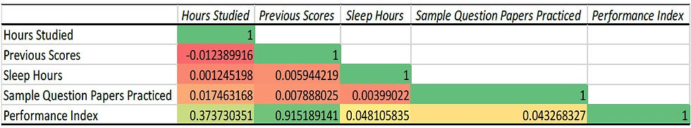
From the above correlation matrix, we see a strong positive correlation of 0.92 between “Previous Scores” (“x” variable) and “Performance Index” (“y” variable).
Let us build the Simple Regression model using “Previous Scores” as the predictor. This technique will help us infer if “Previous Scores” is indeed a cause for variations in “Performance Index”. Next, we split data in 80-20 ratio. So, we consider 8000 records for training the model and remaining 2000 to evaluate it.


Simple Linear Regression Model
The above graph is a scatter plot of “Previous Score” against “Performance Index”. The blue dots are actual data points and the black dotted line is the best fit the linear regression algorithm has found. The Regression analysis output has given us an equation which is nothing but the prediction model.
y= 1.0148x -15.295 which can also be written as
“Performance Index” = 1.0148 * “Previous Score” - 15.295
Model explanation: For every unit change in “Previous Score” the “Performance Index” will change by 1.0148.
R Square value or the Coefficient of determination is 0.8385 or 83.85% which means that the model explains 83.85% of variability in “y” variable.
Root Mean Squared Error or RMSE is an evaluation metrics used in regression problems.
First, we use the model equation to find the predicted value.
Difference between the actual and prediction value is the error.
Next, square the error, find its average and then find its square root.
RMSE is calculated separately for train and test dataset.
For the above case RMSE for train dataset is 7.73 while for test dataset it is 7.78. As RMSE for train and test dataset are not significantly different there is no overfitting problem with the model. (Overfitting issue occurs when model learns minute details from the train data, works very well on it but fails to give good results for test data which is new to it.)
Below chart shows comparison of actual and predicted value of around 30 data points from test dataset:

For the above dataset even with a simple regression model we can explain 83.85% of variation in “Performance Index” and the RMSE comparison show that we have a generalized model available for future prediction.
If we want to further improvise, we start including other predictors or “x” variables and train the model to get multiple linear regression model. While evaluating a multiple regression model there are few assumptions on the data that must be checked and for evaluating the mode we use “Adjusted R Square” value instead of “R Square” value. RMSE is the evaluation metric used in multiple linear regression as well.
The case study thus demonstrates the flow in which we work with data. Define the objective, pick the data, describe it, visualize it, analyse it. Based on the analysis use appropriate algorithms or techniques to derive inferences.


Comments